Introduction:
CONVERGE CFD is being used commercially by many engine and vehicle companies. CONVERGE has an easy to use interface and collection of combustion, spray, and turbulence models which make it an ideal package for simulating gas exchange and combustion for widely varying engines and engine types. EngSim has used the software to simulate two stroke marine diesel engine, 4 stroke gasoline engines, manifold flow, and rotary engine concepts.
One area where EngSim had not seen much work or validation was in external flow simulations. In order to keep one primary 3-D CFD package, EngSim decided to work on some external flow validation studies. With proper validation of simple problems we can move on to full vehicle aerodynamic projects or other general purpose CFD projects. The first simulation problem was to model Karman Vortex Street for a cylinder in cross flow. We then plan to move on to sphere, airfoils, and then full vehicle validation.
The results are very promising.
Geometry:
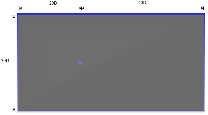
The flow domain is shown in the figure below. The size is sufficient for the full flow development.
Meshing:
The meshing is a critical component of any CFD study, especially Karman Vortex as the eddies form in time and space. The model has embedding around the cylinder with a cell size of 0.5 mm. A box embedding with a cell size of 1 mm was later added to the right of the cylinder to resolve the eddies accurately. A y+ AMR was also added with maximum y + value of 5 and minimum cell size of 0.5. At this refinement level, the model ended up with 142,000 cells (2D domain)
Time step:
The Karman Vortex has a shedding frequency associated with it. This shedding frequency is a function of Reynolds number of the flow. As we were mostly simulating laminar flow cases with low Reynolds number, we chose to use a fixed time step instead of CONVERGE variable time step solver. This proved to be a good approach as we could force large dt without losing the accuracy. It also meant reduction in computation cost by a significant amount. The time step for the current study is 0.0001 seconds.
Solver:
The Karman Vortex problem is generally solved in two steps. First step is to obtain a steady state solution and second step is to use the steady state solution as an initial guess for the transient unsteady solver. The transient solver can be run for a few seconds until the eddies start forming. In this case, we used CONVERGE density based solver to obtain a steady state solution and mapped the solution back to the problem and ran it with transient solver with 0.0001 seconds timesteps.
Boundary Conditions:
1) Velocity boundary condition for the inlet
2) 0 gauge pressure as the boundary condition for the outlet
3) No slip boundary condition over the cylinder
4) Slip boundary condition for the walls on either side
Results:
Drag Force Prediction
CONVERGE reports body forces in X and Y directions. The total body force in X direction gives us the drag coefficient.
CD = Body force in X direction / (0.5 x ρ x V2 x L) ,
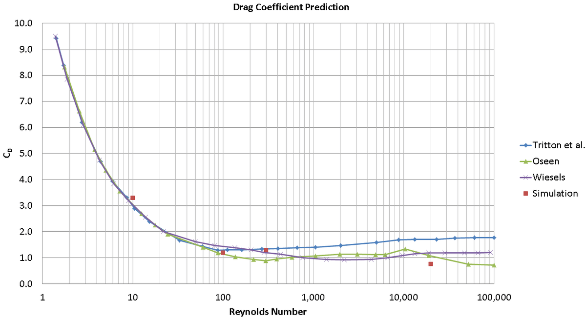
We modeled Re =10, 100, 300 and 20000 flow. For low Reynolds number cases with laminar flow around the cylinder, the CD calculated from simulation agrees with reported values in the literature. The drag prediction at Re =20000 was a little low. The cause may be the standard k-ξ turbulence model we used to model the turbulence, which has been shown to under predict the drag. We plan to investigate different turbulence models in a future study.
Re 10 Drag Prediction:
The flow velocity at Re 10 is a meager 0.014 m/s. Due to this, flow takes considerably longer to develop. This presented an issue as running these simulations for hundreds of seconds was computationally expensive. Hence we ran the simulation for 3.5 seconds and plotted a moving average of the CD. We picked the moving average value at the end of 3.5 seconds. If we run it longer, we might get even closer match. The CD for this case came out to be 3.29.
Re 100 and 300:
The flow at these Reynolds number values became fully steady at or before 5 seconds. Hence time averaging the drag coefficient yielded the correct values of CD.
Re 20000:
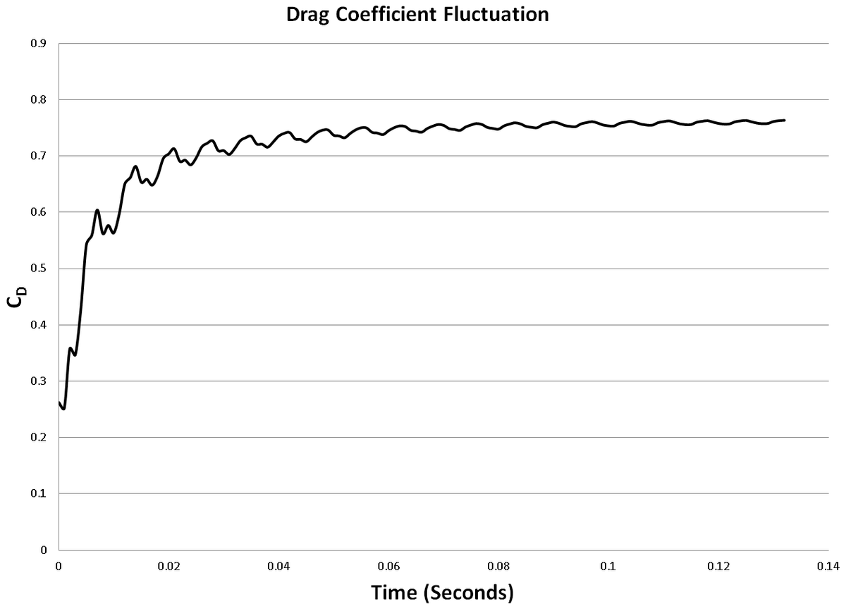
The flow at such high Reynolds number took very little time to develop. The turbulent nature of the flow meant that the flow will never become truly steady. Hence we again used a moving average of the drag coefficient. The CD for this case is 0.76. It was still trending upward slightly but would not have come close to our target value of 1. Running other turbulence models and other Reynolds numbers will give us more information.
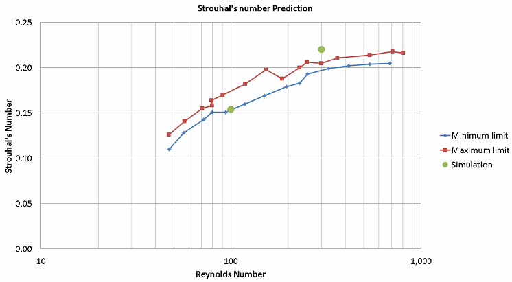
Strouhal’s number:
Strouhal’s number is a function of shedding frequency, characteristic length and velocity and is given by the following equation.
St = (f x L) / V ,
where f is the shedding frequency. Shedding frequency can be defined as the inverse of the time period between two consecutive vortices on the same side of the mean line. Shedding frequency can be calculated from the animation showing the vortex generation.
Re 300 Vortex Formation
Vorticity is a vector quantity and hence it has both magnitude and direction. If we plot the vorticity for all three vortices shown below then we should get a wave with a full period. This is because vorticity reaches its positive peak value for vortex 1, then changes direction and reaches negative peak value for vortex 2 and then changes direction again and reaches positive peak value for vortex 3. In other words, as the vortex 1 and 3 are on the same side of the mean line, the time it takes for vortex 3 to take vortex 1’s place is the shedding period.
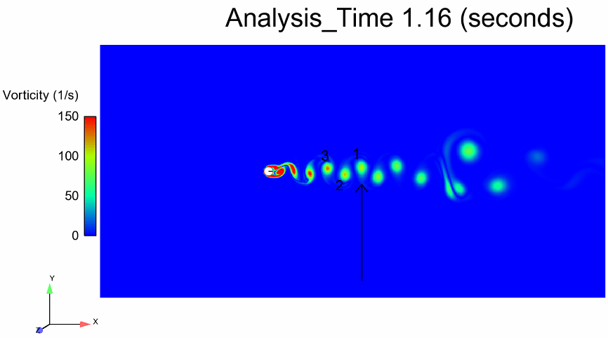
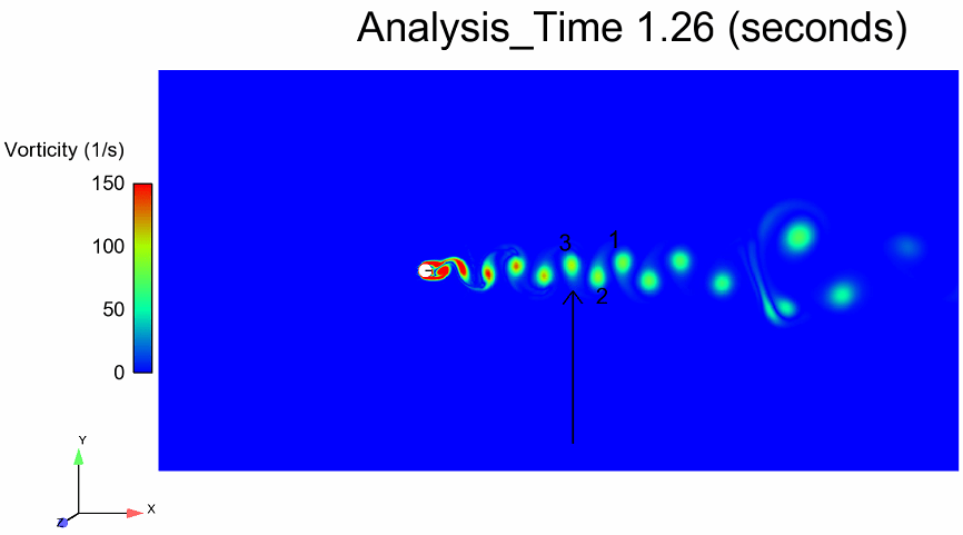
The vortex 3 reaches the same arrow at 1.26 seconds. This means the shedding time period is 0.1 seconds. This gives us the shedding frequency of 10 Hz. Similarly, the shedding period of Re 100 flow was calculated to be 0.43 seconds giving a shedding frequency of 2.32 Hz. We calculated Strouhal’s number for both Reynolds numbers and found them to be agreeing well with the values reported in literature.
Velocity Gradient for Re 300 Flow
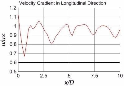
u∞ = Free stream velocity
D = Diameter of Sphere
The x distance for the figure above is measured from center of the sphere. As we move downstream, the flow slows down. In the figure above, the flow reaches its minimum velocity around x/D of 0.5. This is called separation point.This is the point at which the flow viscosity becomes so dominant that the flow cannot move in longitudinal direction anymore. After separation point, the flow velocity starts increasing again.
The peaks in the figure are caused by the vortices whereas the troughs show the gap between two adjacent vortices.
For reference, we have included the vorticity animations for Re=100 and 300 below.
Once the drag prediction for high Reynolds number is improved, EngSim will switch geometries to an airfoil to look at both lift and drag at low and high Reynolds numbers. Once that validation is complete EngSim will be looking for a partner to attempt to validate a full vehicle for lift and drag.
This study was completed by Shreyash Ukidave at EngSim. Please contact him through LinkedIn if you have any questions about the study or CFD capabilities of EngSim.